
Écart x. Attente et variance d'une variable aléatoire
Parmi les nombreux indicateurs utilisés en statistique, il faut souligner le calcul de la variance. Il convient de noter que réaliser ce calcul manuellement est une tâche assez fastidieuse. Heureusement, Excel dispose de fonctions qui permettent d'automatiser la procédure de calcul. Découvrons l'algorithme pour travailler avec ces outils.
La dispersion est un indicateur de variation, qui est le carré moyen des écarts par rapport à l'espérance mathématique. Ainsi, il exprime la répartition des nombres autour de la valeur moyenne. Le calcul de la dispersion peut être effectué soit par population, et de manière sélective.
Méthode 1 : calcul basé sur la population
Pour le calcul cet indicateur dans Excel, la fonction est utilisée pour la population DISP.G. La syntaxe de cette expression est la suivante :
DISP.G(Numéro1;Numéro2;…)
Au total, de 1 à 255 arguments peuvent être utilisés. Les arguments peuvent être soit des valeurs numériques, soit des références aux cellules dans lesquelles ils sont contenus.
Voyons comment calculer cette valeur pour une plage contenant des données numériques.


Méthode 2 : calcul par échantillon
Contrairement au calcul d’une valeur basée sur une population, dans le calcul d’un échantillon, le dénominateur n’indique pas le nombre total de nombres, mais un de moins. Ceci est fait dans le but de corriger les erreurs. Excel prend en compte cette nuance dans une fonction spéciale destinée à ce type de calcul - DISP.V. Sa syntaxe est représentée par la formule suivante :
DISP.B(Numéro1;Numéro2;…)
Le nombre d'arguments, comme dans la fonction précédente, peut également aller de 1 à 255.


Comme vous pouvez le constater, le programme Excel peut grandement faciliter le calcul de la variance. Cette statistique peut être calculée par l'application, soit à partir de la population, soit à partir de l'échantillon. Dans ce cas, toutes les actions de l'utilisateur se résument en réalité à spécifier uniquement la plage de nombres à traiter, et le principal Travail sur Excel le fait lui-même. Bien entendu, cela permettra à l’utilisateur de gagner beaucoup de temps.
Pour les données groupées écart résiduel - moyenne des écarts intragroupe :Où σ 2 j est la variance intragroupe du jème groupe.
Pour les données non groupées écart résiduel– mesure de la précision de l'approximation, c'est-à-dire rapprochement de la droite de régression avec les données originales : 
où y(t) est la prévision utilisant l'équation de tendance ; y t – série dynamique initiale ; n – nombre de points ; p – nombre de coefficients de l'équation de régression (nombre de variables explicatives).
Dans cet exemple, cela s'appelle estimateur de variance sans biais.
Exemple n°1. La répartition des travailleurs de trois entreprises d'une association selon les catégories tarifaires est caractérisée par les données suivantes :
| Catégorie tarifaire travailleur | Nombre de travailleurs dans l'entreprise | ||
| entreprise 1 | entreprise 2 | entreprise 3 | |
| 1 | 50 | 20 | 40 |
| 2 | 100 | 80 | 60 |
| 3 | 150 | 150 | 200 |
| 4 | 350 | 300 | 400 |
| 5 | 200 | 150 | 250 |
| 6 | 150 | 100 | 150 |
Définir:
1. écart pour chaque entreprise (écarts intra-groupe) ;
2. la moyenne des écarts intra-groupe ;
3. dispersion intergroupes ;
4. variance totale.
Solution.
Avant de commencer à résoudre le problème, il est nécessaire de savoir quelle fonctionnalité est efficace et laquelle est factorielle. Dans l'exemple considéré, l'attribut résultant est « Catégorie tarifaire » et l'attribut facteur est « Numéro (nom) de l'entreprise ».
On a alors trois groupes (entreprises), pour lesquels il faut calculer la moyenne du groupe et les variances intragroupe :
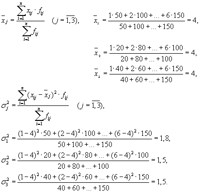
| Entreprise | Moyenne du groupe, | Variation au sein du groupe, |
| 1 | 4 | 1,8 |
La moyenne des variances intra-groupe ( écart résiduel) sera calculé à l'aide de la formule :

où l'on peut calculer :

ou:
Alors:
La variance totale sera égale à : s 2 = 1,6 + 0 = 1,6.
La variance totale peut également être calculée à l'aide de l'une des deux formules suivantes :
Lors de la résolution de problèmes pratiques, on est souvent confronté à une caractéristique qui ne prend que deux valeurs alternatives. Dans ce cas, nous ne parlons pas du poids d'une valeur particulière d'une caractéristique, mais de sa part dans la totalité. Si la proportion d’unités de population possédant la caractéristique étudiée est désignée par « r", et ceux qui n'en ont pas - via " q", alors la variance peut être calculée à l'aide de la formule :
s 2 = p×q
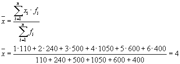
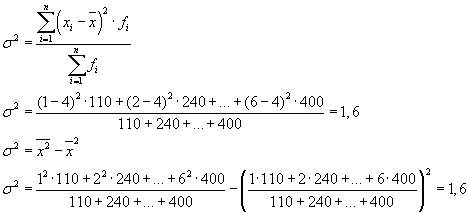
Exemple n°2. À partir des données de production de six travailleurs d'une équipe, déterminez la variance intergroupe et évaluez l'impact du quart de travail sur leur productivité du travail si la variance totale est de 12,2.
| Travailleur d'équipe n° | Production des travailleurs, pcs. | |
| dans le premier quart de travail | dans le deuxième quart de travail | |
| 1 | 18 | 13 |
| 2 | 19 | 14 |
| 3 | 22 | 15 |
| 4 | 20 | 17 |
| 5 | 24 | 16 |
| 6 | 23 | 15 |
Solution. Données initiales
| X | f1 | f2 | f3 | f4 | f5 | f6 | Total |
| 1 | 18 | 19 | 22 | 20 | 24 | 23 | 126 |
| 2 | 13 | 14 | 15 | 17 | 16 | 15 | 90 |
| Total | 31 | 33 | 37 | 37 | 40 | 38 |
Nous avons ensuite 6 groupes pour lesquels il faut calculer la moyenne de groupe et les variances intragroupe.
1. Trouvez les valeurs moyennes de chaque groupe.
2. Trouvez le carré moyen de chaque groupe.
Résumons les résultats du calcul dans un tableau :
| Numéro de groupe | Moyenne du groupe | Variation au sein du groupe |
| 1 | 1.42 | 0.24 |
| 2 | 1.42 | 0.24 |
| 3 | 1.41 | 0.24 |
| 4 | 1.46 | 0.25 |
| 5 | 1.4 | 0.24 |
| 6 | 1.39 | 0.24 |
3. Variation au sein du groupe caractérise le changement (variation) de la caractéristique étudiée (résultative) au sein d'un groupe sous l'influence de tous les facteurs sur celui-ci, à l'exception du facteur sous-jacent au regroupement :
La moyenne des écarts intragroupe sera calculée selon la formule :
4. Variation intergroupe caractérise le changement (variation) de la caractéristique étudiée (résultative) sous l'influence d'un facteur (caractéristique factorielle) qui constitue la base du groupe.
Nous définissons la variance intergroupe comme :
Où
Alors
Écart total caractérise le changement (variation) de la caractéristique étudiée (résultative) sous l'influence de tous les facteurs (caractéristiques factorielles) sans exception. Selon les conditions du problème, elle est égale à 12,2.
Relation de corrélation empirique mesure quelle partie de la variabilité totale de la caractéristique résultante est causée par le facteur étudié. Il s’agit du rapport entre la variance factorielle et la variance totale :
Nous définissons la relation de corrélation empirique :
Les liens entre les caractéristiques peuvent être faibles et forts (étroits). Leurs critères sont évalués sur l'échelle de Chaddock :
0,1 0,3 0,5 0,7 0,9 Dans notre exemple, la relation entre le trait Y et le facteur X est faible
Coefficient de détermination.
Déterminons le coefficient de détermination :
Ainsi, 0,67 % de la variation est due à des différences entre les caractères, et 99,37 % est due à d'autres facteurs.
Conclusion: dans ce cas, la production des travailleurs ne dépend pas du travail effectué lors d'un quart de travail spécifique, c'est-à-dire l'influence du quart de travail sur la productivité du travail n'est pas significative et est due à d'autres facteurs.
Exemple n°3. Basé sur une moyenne salaires et les écarts au carré de sa valeur pour deux groupes de travailleurs, trouvez la variance totale en appliquant la règle d'addition des variances :
Solution:Moyenne des écarts intra-groupe
Nous définissons la variance intergroupe comme :
La variance totale sera : 480 + 13824 = 14304
Cette page décrit un exemple standard de recherche de variance, vous pouvez également examiner d'autres problèmes pour la trouver.
Exemple 1. Détermination du groupe, de la moyenne du groupe, de l'intergroupe et de la variance totale
Exemple 2. Trouver la variance et le coefficient de variation dans un tableau de regroupement
Exemple 3. Trouver la variance dans série discrète
Exemple 4. Les données suivantes sont disponibles pour un groupe de 20 étudiants par correspondance. Il faut construire série d'intervalles distribution d'une caractéristique, calculer la valeur moyenne de la caractéristique et étudier sa variance
Construisons un regroupement d'intervalles. Déterminons la plage de l'intervalle à l'aide de la formule :
![]()
où X max est la valeur maximale de la caractéristique de regroupement ;
X min – valeur minimale de la caractéristique de regroupement ;
n – nombre d'intervalles :
Nous acceptons n=5. Le pas est : h = (192 - 159)/ 5 = 6,6
Créons un regroupement d'intervalles

Pour d'autres calculs, nous construirons un tableau auxiliaire :

X"i – le milieu de l'intervalle. (par exemple, le milieu de l'intervalle 159 – 165,6 = 162,3)
Nous déterminons la taille moyenne des élèves à l'aide de la formule de moyenne arithmétique pondérée :

Déterminons la variance à l'aide de la formule :
La formule peut être transformée comme ceci :

De cette formule il résulte que la variance est égale à la différence entre la moyenne des carrés des options et le carré et la moyenne.
Dispersion dans les séries de variationsà intervalles égaux en utilisant la méthode des moments peut être calculé de la manière suivante en utilisant la deuxième propriété de dispersion (en divisant toutes les options par la valeur de l'intervalle). Détermination de l'écart, calculé selon la méthode des moments, la formule suivante est moins laborieuse :

où i est la valeur de l'intervalle ;
A est un zéro conventionnel, pour lequel il convient d'utiliser le milieu de l'intervalle de fréquence la plus élevée ;
m1 est le carré du moment du premier ordre ;
m2 - moment du deuxième ordre
Variance des traits alternatifs (si dans une population statistique une caractéristique change de telle manière qu'il n'y a que deux options mutuellement exclusives, alors cette variabilité est appelée alternative) peut être calculée à l'aide de la formule :

En substituant q = 1- p dans cette formule de dispersion, nous obtenons :

Types de variance
Écart total mesure la variation d’une caractéristique dans l’ensemble de la population sous l’influence de tous les facteurs qui provoquent cette variation. Il est égal au carré moyen des écarts valeurs individuelles caractéristique x à partir de la moyenne globale de x et peut être définie comme une variance simple ou une variance pondérée.
Variation au sein du groupe caractérise la variation aléatoire, c'est-à-dire partie de la variation qui est due à l'influence de facteurs non pris en compte et ne dépend pas de l'attribut facteur qui constitue la base du groupe. Une telle dispersion est égale au carré moyen des écarts des valeurs individuelles de l'attribut au sein du groupe X par rapport à la moyenne arithmétique du groupe et peut être calculée comme une dispersion simple ou comme une dispersion pondérée.
Ainsi, mesures de variance au sein du groupe variation d'un trait au sein d'un groupe et est déterminé par la formule :

où xi est la moyenne du groupe ;
ni est le nombre d'unités dans le groupe.
Par exemple, les variances intragroupe qui doivent être déterminées dans le cadre de l'étude de l'influence des qualifications des travailleurs sur le niveau de productivité du travail dans un atelier montrent des variations de production dans chaque groupe causées par tous les facteurs possibles (état technique de l'équipement, disponibilité des équipements). outils et matériaux, âge des travailleurs, intensité de travail, etc.), à l'exception des différences de catégorie de qualification (au sein d'un groupe, tous les travailleurs ont les mêmes qualifications).
Selon l’enquête par sondage, les déposants ont été regroupés selon le montant de leur dépôt à la Sberbank de la ville :
Définir:
1) étendue des variations ;
2) taille moyenne des dépôts ;
3) moyenne déviation linéaire;
4) dispersion ;
5) écart type ;
6) coefficient de variation des cotisations.
Solution:
Cette série de distribution contient des intervalles ouverts. Dans de telles séries, la valeur de l'intervalle du premier groupe est classiquement supposée égale à la valeur de l'intervalle du suivant, et la valeur de l'intervalle du dernier groupe est égale à la valeur de l'intervalle du le précédent.
La valeur de l'intervalle du deuxième groupe est égale à 200, donc la valeur du premier groupe est également égale à 200. La valeur de l'intervalle de l'avant-dernier groupe est égale à 200, ce qui signifie que le dernier intervalle sera également ont une valeur de 200.
1) Définissons la plage de variation comme la différence entre la plus grande et la plus petite valeur de l'attribut :
La plage de variation du montant du dépôt est de 1 000 roubles.
2) Le montant moyen de la contribution sera déterminé à l'aide de la formule de la moyenne arithmétique pondérée.
Déterminons d'abord quantité discrète fonctionnalité dans chaque intervalle. Pour ce faire, en utilisant la formule simple de la moyenne arithmétique, nous trouvons les milieux des intervalles.
La valeur moyenne du premier intervalle sera :

le second - 500, etc.
Entrons les résultats du calcul dans le tableau :
| Montant du dépôt, frotter. | Nombre de déposants, f | Milieu de l'intervalle, x | xf |
|---|---|---|---|
| 200-400 | 32 | 300 | 9600 |
| 400-600 | 56 | 500 | 28000 |
| 600-800 | 120 | 700 | 84000 |
| 800-1000 | 104 | 900 | 93600 |
| 1000-1200 | 88 | 1100 | 96800 |
| Total | 400 | - | 312000 |
Le dépôt moyen à la Sberbank de la ville sera de 780 roubles :
3) L'écart linéaire moyen est la moyenne arithmétique des écarts absolus des valeurs individuelles d'une caractéristique par rapport à la moyenne globale :

La procédure de calcul de l'écart linéaire moyen dans la série de distributions d'intervalles est la suivante :
1. La moyenne arithmétique pondérée est calculée comme indiqué au paragraphe 2).
2. Les écarts absolus par rapport à la moyenne sont déterminés :
3. Les écarts résultants sont multipliés par les fréquences :
4. Trouver la somme des écarts pondérés sans tenir compte du signe :
5. La somme des écarts pondérés est divisée par la somme des fréquences :
Il est pratique d'utiliser le tableau des données de calcul :
| Montant du dépôt, frotter. | Nombre de déposants, f | Milieu de l'intervalle, x | |||
|---|---|---|---|---|---|
| 200-400 | 32 | 300 | -480 | 480 | 15360 |
| 400-600 | 56 | 500 | -280 | 280 | 15680 |
| 600-800 | 120 | 700 | -80 | 80 | 9600 |
| 800-1000 | 104 | 900 | 120 | 120 | 12480 |
| 1000-1200 | 88 | 1100 | 320 | 320 | 28160 |
| Total | 400 | - | - | - | 81280 |

L'écart linéaire moyen du montant du dépôt des clients de la Sberbank est de 203,2 roubles.
4) La dispersion est la moyenne arithmétique des carrés des écarts de chaque valeur d'attribut par rapport à la moyenne arithmétique.
Le calcul de la variance dans les séries de distributions d'intervalles est effectué à l'aide de la formule :

La procédure de calcul de l'écart dans ce cas est la suivante :
1. Déterminez la moyenne arithmétique pondérée, comme indiqué au paragraphe 2).
2. Trouvez les écarts par rapport à la moyenne :
3. Mettez au carré l’écart de chaque option par rapport à la moyenne :
4. Multipliez les carrés des écarts par les poids (fréquences) :
![]()
5. Résumez les produits obtenus :
![]()
6. Le montant obtenu est divisé par la somme des poids (fréquences) :

Mettons les calculs dans un tableau :
| Montant du dépôt, frotter. | Nombre de déposants, f | Milieu de l'intervalle, x | |||
|---|---|---|---|---|---|
| 200-400 | 32 | 300 | -480 | 230400 | 7372800 |
| 400-600 | 56 | 500 | -280 | 78400 | 4390400 |
| 600-800 | 120 | 700 | -80 | 6400 | 768000 |
| 800-1000 | 104 | 900 | 120 | 14400 | 1497600 |
| 1000-1200 | 88 | 1100 | 320 | 102400 | 9011200 |
| Total | 400 | - | - | - | 23040000 |
Dispersion dans les statistiques se trouve comme les valeurs individuelles de la caractéristique au carré de . En fonction des données initiales, elle est déterminée à l'aide des formules de variance simples et pondérées :
1. (pour les données non groupées) est calculé à l'aide de la formule :
2. Variance pondérée (pour les séries de variations) :
 où n est la fréquence (répétabilité du facteur X)
Un exemple de recherche de variance
Cette page décrit un exemple standard de recherche de variance, vous pouvez également examiner d'autres problèmes pour la trouver.
Exemple 1. Les données suivantes sont disponibles pour un groupe de 20 étudiants par correspondance. Il est nécessaire de construire une série d'intervalles de distribution de la caractéristique, de calculer la valeur moyenne de la caractéristique et d'étudier sa dispersion
 Construisons un regroupement d'intervalles. Déterminons la plage de l'intervalle à l'aide de la formule :
![]() où X max est la valeur maximale de la caractéristique de regroupement ;
où X max est la valeur maximale de la caractéristique de regroupement ;
X min – valeur minimale de la caractéristique de regroupement ;
n – nombre d'intervalles :
Nous acceptons n=5. Le pas est : h = (192 - 159)/ 5 = 6,6
Créons un regroupement d'intervalles
 Pour d'autres calculs, nous construirons un tableau auxiliaire :
 X'i est le milieu de l'intervalle. (par exemple, le milieu de l'intervalle 159 – 165,6 = 162,3)
Nous déterminons la taille moyenne des élèves à l'aide de la formule de moyenne arithmétique pondérée :
 Déterminons la variance à l'aide de la formule :
La formule de dispersion peut être transformée comme suit :

De cette formule il résulte que la variance est égale à la différence entre la moyenne des carrés des options et le carré et la moyenne.
Dispersion dans les séries de variationsà intervalles égaux en utilisant la méthode des moments peut être calculé de la manière suivante en utilisant la deuxième propriété de dispersion (en divisant toutes les options par la valeur de l'intervalle). Détermination de l'écart, calculé selon la méthode des moments, la formule suivante est moins laborieuse :

où i est la valeur de l'intervalle ;
A est un zéro conventionnel, pour lequel il convient d'utiliser le milieu de l'intervalle de fréquence la plus élevée ;
m1 est le carré du moment du premier ordre ;
m2 - moment du deuxième ordre
(si dans une population statistique une caractéristique change de telle manière qu'il n'y a que deux options mutuellement exclusives, alors cette variabilité est appelée alternative) peut être calculée à l'aide de la formule :

En substituant q = 1- p dans cette formule de dispersion, nous obtenons :

Types de variance
Écart total mesure la variation d’une caractéristique dans l’ensemble de la population sous l’influence de tous les facteurs qui provoquent cette variation. Elle est égale au carré moyen des écarts des valeurs individuelles d'une caractéristique x par rapport à la valeur moyenne globale de x et peut être définie comme variance simple ou variance pondérée.
caractérise la variation aléatoire, c'est-à-dire partie de la variation qui est due à l'influence de facteurs non pris en compte et ne dépend pas de l'attribut facteur qui constitue la base du groupe. Une telle dispersion est égale au carré moyen des écarts des valeurs individuelles de l'attribut au sein du groupe X par rapport à la moyenne arithmétique du groupe et peut être calculée comme une dispersion simple ou comme une dispersion pondérée.
Ainsi, mesures de variance au sein du groupe variation d'un trait au sein d'un groupe et est déterminé par la formule :

où xi est la moyenne du groupe ;
ni est le nombre d'unités dans le groupe.
Par exemple, les variances intragroupe qui doivent être déterminées dans le cadre de l'étude de l'influence des qualifications des travailleurs sur le niveau de productivité du travail dans un atelier montrent des variations de production dans chaque groupe causées par tous les facteurs possibles (état technique de l'équipement, disponibilité des équipements). outils et matériaux, âge des travailleurs, intensité de travail, etc.), à l'exception des différences de catégorie de qualification (au sein d'un groupe, tous les travailleurs ont les mêmes qualifications).
La moyenne des variances au sein du groupe reflète le hasard, c'est-à-dire la partie de la variation qui s'est produite sous l'influence de tous les autres facteurs, à l'exception du facteur de regroupement. Il est calculé à l'aide de la formule :

Caractérise la variation systématique de la caractéristique résultante, qui est due à l'influence du facteur-signe qui constitue la base du groupe. Il est égal au carré moyen des écarts des moyennes de groupe par rapport à la moyenne globale. La variance intergroupe est calculée à l'aide de la formule :

La règle pour ajouter de la variance dans les statistiques
Selon règle d'ajout d'écarts la variance totale est égale à la somme de la moyenne des variances intra-groupe et inter-groupes :
![]()
Le sens de cette règle est que la variance totale résultant de l'influence de tous les facteurs est égale à la somme des variances résultant de l'influence de tous les autres facteurs et de la variance résultant du facteur de regroupement.
À l'aide de la formule d'addition de variances, vous pouvez déterminer la troisième variance inconnue à partir de deux variances connues et également juger de la force de l'influence de la caractéristique de regroupement.
Propriétés de dispersion
1. Si toutes les valeurs d'une caractéristique sont réduites (augmentées) du même montant constant, alors la dispersion ne changera pas.
2. Si toutes les valeurs d'une caractéristique sont réduites (augmentées) du même nombre de fois n, alors la variance diminuera (augmentera) en conséquence de n^2 fois.